
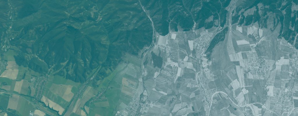
Historical Canopy Gap Analysis in Old-Growth Beech Forests
Investigating canopy structure and disturbance patterns in the Havešová old-growth reserve in 1975.
Use case
RETROCANOPY
Author
Ladislav Šumichrast
Institution
Technical University in Zvolen, Slovakia
Research areas
Forest disturbance ecology; old-growth forests; canopy dynamics; historical remote sensing; spatial analysis
Study area
Havešová old-growth reserve, Poloniny National Park, Slovakia · 144.7 ha
Reference period
1975
Research question
What can a single historical satellite image reveal about small canopy openings and the disturbance pattern of a beech old-growth forest?
Overview
Small disturbances in old-growth beech forests can open the canopy without producing a clear forest/non-forest change. This use case examines these finer features in a single KH-9 Hexagon image of Havešová from 1975.
The notebook corrects broad differences in illumination and identifies dark canopy features under a documented detection rule and minimum area. It then describes their extent, sizes, spatial arrangement and distances to the surrounding canopy. The delivered example includes visual checks, sensitivity analyses and a recorded manual correction.
Inputs and workflow
What you need
- An orthorectified panchromatic raster clipped to the study area, with explicit NoData outside it.
- The supplied Havešová raster has a 0.5 m grid in EPSG:5514.
- For exact reproduction of the example, the supplied correction polygon and all its Shapefile components. The gap analysis itself requires no elevation model or field plots.
Main steps
- Load the clipped raster, verify its mask and inspect image quality.
- Correct local illumination differences and inspect the detection-rule preview.
- Apply the chosen threshold, minimum area and documented cleanup rules.
- Review candidate features and record any manual corrections.
- Generate maps and statistics, inspect sensitivity to the detection choices, and report the settings with the results.
What you get
- Maps of canopy-gap candidates and their share of the analysed reserve.
- Size distributions, density and spatial-arrangement statistics, plus distances to detected openings.
- Sensitivity tables, figures and processing records; browser-readable versions of the worked example.
Demonstrated example
Under the documented rule, the Havešová example maps dark canopy depressions covering 13.96% of the analysed reserve: approximately 20.2 ha out of 144.7 ha. Most detected features are small. The reported result includes the supplied manual correction and must be interpreted together with the threshold and minimum mapped area.
Interpretation and limits
Shadow is a proxy for canopy structure. A single panchromatic image cannot establish a height-based ecological gap definition or distinguish every true opening from a height difference between crowns. These are canopy-gap candidates rather than ground-confirmed gaps.
Their measured extent depends on the detection convention; the example is a single-date baseline, not a disturbance chronology.
Video demonstration
A recorded explanation of the image constraints, detection method, Havešová example and sensitivity of the interpretation.
Materials
Workflow package
The analysis notebook, environment definition and Python requirements for reproducing the workflow.
Havešová 1975 GeoTIFF and the manual correction dataset. Keep all Shapefile components together to reproduce the supplied example.
User guide and worked example
Method, input requirements, detection settings and interpretation, with browser-readable results from the Havešová example.
Download user guide (PDF)Presentation
The scientific question, image constraints, detection method and results from Havešová.
Download presentation (PDF)How to reuse this use case
Use the notebook to explore historical canopy structure in comparable closed-canopy forest images. Replace the raster, review the detection settings and inspect sensitivity before interpreting the results. The supplied correction polygon belongs to Havešová and should be disabled or replaced for a new area. The documentation describes local Jupyter and EOSC EU Node operation.
When reporting results, identify the input datasets and acquisition dates, the workflow version, processing settings and evaluation scope. Keep the documentation with the files you reuse and follow the license supplied with each resource.